Automatic market-makers (AMMs) are one of the major innovations which decentralized finance has brought. They use the maths function to price assets when exchanging two or more tokens. First, Uniswap brought markets created by $x·y = k$ invariant which doesn’t make any assumption about the pricing of underlying assets and spreads liquidity across all prices evenly. Next, Curve introduced the stableswap invariant which allowed to focus most of the liquidity around price 1.0, a very useful feature for creating stablecoin-to-stablecoin liquidity.
Since the inception of AMMs, there have been several notable improvements in AMMs. One such improvement is Curve V2 which introduced CurveCrypto Invariant and can be used to create liquidity for tokens that are not necessarily pegged to each other i.e. their price changes frequently w.r.t. each other.
Limitation of AMMs in Leverage Trading
All these innovations work perfectly fine when it comes to token swaps but it is difficult to apply the same to derivatives, such as perpetual futures. As derivative trading involves leverage, the position value will be bounded by the pool size, and also the liquidity providers might suffer from high impermanent loss.
To overcome this problem, Perpetual protocol introduced the concept of Virtual AMMs or vAMMs. As the “virtual” part of vAMM implies, there is no real asset pool stored inside the vAMM itself. Instead, the real asset is stored in a smart contract vault that manages all of the collateral backing the vAMM; and the vAMM is just used for pricing the perps. In fact, that is how the Mark Price is determined. The perpetual protocol uses $x*y = k$ (Uniswap v2) invariant in their vAMM. Perpetual protocol V2 is planned to be utilizing the Uniswap V3 which relies on makers who provide liquidity around tight ranges and move liquidity accordingly as price changes.
Hubble vAMM
At Hubble, we are using CurveCrypto Invariant in our vAMM. As described in Curve V2 whitepaper, it is way more efficient than $x · y = k$ invariant and concentrates liquidity given by the current “internal oracle” price but only moves that price when the loss is smaller than part of the profit which the system makes. This creates 5 − 10 times higher liquidity than the Uniswap invariant.
Here is an example of how it works under the hood.
- Before starting any trade, we add virtual liquidity to the pool and set the initial rate. Let say we have a vUSDT/vETH pool with 1,000,000 vUSDT and 1000 vETH initially, setting the initial vETH price 1000 vUSDT.
- Alice adds 1000 USDT to the smart contract vault as margin and wants to long 5 ETH i.e. 5x leverage. The protocol calculates the amount of vUSDT required to buy 5 vETH using CurveCrypto invariant and adds the same to the vAMM pool and removes the 5 vETH from it. The final state of the pool after the transaction is 995 vETH and 1,005,008.997 vUSDT.
- Another trader Bob also adds a 1000 USDT margin and wants to short 5 ETH i.e. 5x leverage. The protocol calculates the amount of vUSDT required to sell 5 vETH using CurveCrypto invariant and removes the same from the vAMM pool and adds the 5 vETH to it. The final state of the pool after the transaction is 1000 vETH and 1,000,000 vUSDT.
Unique Properties of Hubble vAMM
Repegging
In contrast to Uniswap V3, Curve V2 uses an internal oracle to concentrate liquidity and the repegging algorithm takes care of the price update. This makes our vAMM ‘smart’ enough to concentrate liquidity around the current price by itself.
Since Curve V2 is not path independent, there is a need for Makers in the system to counter the profit/loss due to that. Makers add virtual liquidity to the pool on leverage and earn a part of the trading fee. The good part is, makers don’t have to worry about the price range in which they have to provide liquidity to deepen the liquidity around the current price. The repegging algorithm deepens liquidity around current price automatically and hence makers earn fee regardless of the price change. During highly volatile market, makers don’t have to worry about getting out of range and lose out on pool fee.
Maths behind Hubble vAMM
The main advantage of using this vAMM is that the repegging algorithm takes care of liquidity concentration around the current price.
Repegging Algorithm
The repegging profit/loss is quantified by constant-product invariant at the equilibrium point. For a pool with $n$ tokens, it is given as
$$ X_{c p}=\left(\prod \frac{D}{n p_{i}}\right)^{\frac{1}{n}} $$
where D is the total value of the pool in the terms of the base token (0th token) when the pool is in equilibrium and $p_i$ is the price of the $i^{th}$ token. When we change $p$, the price peg changes but balances don’t. We can calculate the new $D$ for the new values of $p$ and substitute new $D$ and $p_i$ to calculate $X_{cp}$.
We track $X_{cp}$ at every exchange or deposit. We also track the $virtual_price = X_{cp}/total\_supply$, where $total\_supply$ is the virtual LP token supply. It keeps track of all the losses after $p$ adjustments. Note that, since it is a vAMM, neither there are actual LP tokens minted nor any fee is charged inside the vAMM. It is used just for calculation purposes.
After every operation, we multiply a variable xcp_profit by virtual_price/old_virtual_price, starting with $1.0$. We undo the price adjustment if it causes virtual_price-1 to fall lower than half of xcp_profit-1.
Internally, we have a price oracle given by an exponential moving average applied in N-dimensional price space. Suppose that the last reported price is
$p_{last}$, and the update happened $t$ seconds ago while the half-time of the EMA is $T_{1/2}$. Then the oracle price $p^*$ is given as:
$$ \alpha=2^{-\frac{t}{T_{1 / 2}}} $$ $$ \mathbf{p}^{*}=\mathbf{p}_{l a s t}(1-\alpha)+\alpha \mathbf{p}_{prev}^{*} $$
CurveCrypto Invariant
This invariant is encouraged by the StableSwap invariant. For a pool with $n$ number of coins, it is represented as
$$ \begin{equation} KD^{n-1}\sum x_i = KD^n + \bigg(\frac{D}{n}\bigg)^n \end{equation} $$
$$ \begin{equation} K = AK_0\frac{\gamma^2}{\big(\gamma+1-K_0\big)^2}, \hskip{2em} K_0 = \frac{\prod x_i n^n}{D^n} \end{equation} $$
where $x_i$ represents the balance of $i^{th}$token, $D = nx_{eq}$ is the total deposits in the pool when it is in equilibrium, $A$ is amplification coefficient, and $\gamma > 0$ is usually a small number. Figure 1 shows the graph of equation (1) and its comparison with the constant product ($xy =k$) and stable swap invariant.
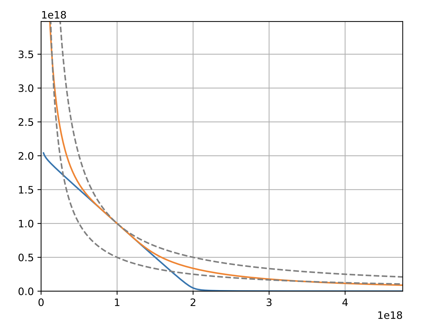
Figure 1: Comparison of AMM invariants: constant-product (dashed line), stable swap (blue), and curve crypto invariant (orange)
Figure 1: Comparison of AMM invariants: constant-product (dashed line), stable swap (blue), and curve crypto invariant (orange) Image source: https://curve.fi/files/crypto-pools-paper.pdf
Check out this notebook to know more about the effects of varying $A$ or $\gamma$ on the curve. To get the amount of output token ($x_j$), given input token amount ($x_i$), equation (1) needs to be solved for $x_j$ by Newton’s method.
Swapping Tokens (newton_y)
Suppose a trader wants to swap $dx$ amount of token $i$ for token $j$. The amount of token to be received by the trader $dy = y_{initial} - y_{new}$, where $y_{initial}$ is the balance of token $x_j$ before this trade and $y_{new}$ is calculated by solving the equation (1) for $x_j = y$, given all other parameters are known. We need to find the roots of the equation
$$ \begin{equation} f(y) = KD^{n-1}\sum x_i + \prod x_i - KD^n - \bigg(\frac{D}{N}\bigg)^n = 0 \end{equation} $$
Substituting $S = \sum x_i = \sum_{i \not= j}^{n} x_i + y$, $\prod x_i = y\prod_{i \not= j}^n x_i = \frac{K_0D^n}{n^n}$, $K$ from equation (2), and $Ann = An^n$ in the above equation gives
$$ \begin{equation} f(y) = S-D + \frac{D(K_0-1)(\gamma+1-K_0)^2}{AnnK_0\gamma^2} = 0 \end{equation} $$
Using $S' = 1$ and $K_0' = \frac{K_0}{y}$, the derivative of $f(y)$ can be represented as
$$ \begin{equation} y_nf'(y_n) = y_n + \frac{D(\gamma+1-K_0)^2}{Ann\gamma^2} + S\bigg(\frac{2K_0}{\gamma+1-K_0}+1\bigg) - D\bigg(\frac{2K_0}{\gamma+1-K_0}+1\bigg) \end{equation} $$
Finally, $y_{new}$ can be calculated by finding the root of equation (4) by iterating the below equation until convergence.
$$ \begin{equation} y_{n+1} = y_n - \frac{f(y_n)}{f'(y_n)} = \frac{y_nf'(y_n)-f(y_n)}{f'(y_n)} \end{equation} $$
Check out the implementation of the above algorithm in the newton_y(Ann,gamma,x,D,i) function of Curve’s math contract.
Similarly, newton_D(ANN, gamma, x) is used to calculate $D$ given A, gamma, and balances $x$.